Building an embedded device for sailboat racing: the software

This is the fourth post in a series about building an embedded electronic device to assist in sailboat racing.

Marine electronics project — table of contents

1. Project background
2. The platform
3. A digression on suppliers…
4. The software
5. Power and packaging
6. Fabrication and assembly
7. Mounting and installation (take one)
8. Installation (take two) — Success!

With the basic platform package chosen — Raspberry Pi, a 7″ 800×480 sunlight-readable touchscreen, and the NGT-1 — it was time to put it to work. This post dives into the software built to run on this platform and deliver that telemetry analysis and visualization I was looking for.

Communicating with NMEA2000

The first order of business is communicating with the NMEA2000 data network that links all my instruments together. As mentioned, the Actisense NGT-1 is a network gateway/bridge that speaks N2K on one side, and emulates a serial port via USB on the other side. Actisense also has an SDK that will let you integrate it into your project. It’s not available for download on their web site; you need to file a support ticket with them and ask for it, but they will give it to you for free. Unfortunately, to use this SDK I needed to sign an NDA, which makes it cumbersome to share the source code for this project. (If enough folks are interested, I might do the work to separate out the codebase that’s definitely mine from the parts that work directly with their “ACCompLib” drivers…)

Their SDK contains a few different components, including demo apps written in C# (helpful to study, especially if you want to develop on Windows), as well as a lower-level driver library. They’re primarily Windows-centric, which was a mild hurdle to overcome, but the base library is in C and they provide access to the source code, so it was still possible to use it in Linux. They also provided some quite good SDK developer documentation. I had to write Makefiles to build their library and make a few other tweaks so that it was gcc-friendly, but the changes were minimally invasive.

Beyond that, some simple choices from Actisense made things a tad cumbersome on Linux. Take for example the name: “ACCompLib.” (For “Actisense Component Library”, maybe?) I initially got the Makefile to build it and produce a file named ACCompLib.so, but then actually linking it into my project was hard; Linux really wants your shared libraries to be named libfoo.so, not foolib.so, and definitely not FooLib.so; when you compile your project you need to invoke this with something like gcc myprgm.c -o myprgm.o -lfoo; it will then search for libfoo.so, and using complete filenames rather than this “library nickname” style is discouraged. So the binary image’s name had to change around to libaccomp.so .

ACCompLib is also a very low-level library that focuses on controlling the NGT-1; it has APIs to read and write N2K messages but also several other APIs that configure and monitor the NGT-1 itself out-of-band from the N2K message stream; I had to write another layer on top of this library to add a message queue that let me stack up the messages and process them one at a time in my application, but that wasn’t too much trouble (and refreshed my knowledge of pthreads in the process). After that, I used Boost.Python to wrap my higher-level library in a Python class, which opened up the path to developing the rest of the system in Python.

Finally, the NGT-1 manifests as a character stream device to Linux; I added a udev rule to recognize this particular device and make it visible at /dev/NGT1 so it would always be available at a standard path to my application.

Making a dashboard UI

My main goal for the project was clarity. I wanted to be able to glance at this device quickly, and instantly know what to do, so I could get back to focusing on sailing. For bonus points, I wanted it to “fit in” with other sailing device interfaces and have a similar look-and-feel to my MFD.

Finally, since I had bought a touchscreen (and ruled out additional buttons to avoid adding holes in the case that might leak water), all the interaction would be through icon-based buttons. I also wanted as few of these as possible, so that I hopefully didn’t need to directly interact with it at all during a race. While it would offer some configuration capabilities, normal usage would be purely passive.

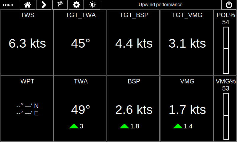
I eventually converged on a set of ten “digital dashboard elements” arranged as above. The true wind speed (TWS) is shown in the upper left, and that is the “key” to the current targets, shown to the right: TGT_TWA is the target true wind angle, TGT_BSP is the target boatspeed, and TGT_VMG is the VMG you would achieve if sailing at that speed along that angle to the wind (VMG = BSP * cos(TWA)). The lower row shows the current waypoint (none set in this screenshot), and the actual TWA, BSP, and VMG values, each aligned below its target.

Displaying these next to one another is a pretty clear picture but even then you still need to compare the numbers and do some minor mental arithmetic. The smaller numbers (and triangle icons) read it out as simple directions: in the TWA box it is saying “head further upwind 3 degrees.” The BSP box says “increase speed by 1.8 kts,” and the VMG box says “increase VMG by 1.4 kts.” Those can also be red triangles for head downwind / decelerate, or blue squares meaning “hold here” if the delta between actual and target values is close to zero.

On the right are two “progress bars” that show the current speed as a % of the polar speed (in POL%) and the current VMG as a % of its target below that. As you can see, when I was capturing demo data to replay for this example, at least at this particular moment I wasn’t sailing very efficiently at all!

Finally, at the top of the view you can see some buttons to advance between screens or flip to the settings view, etc. The words “Upwind performance” indicate the mode the device is operating in. In order to calculate VMG, you need to know where the boat is trying to get to. If you set a course to navigate by waypoints on your chartplotter, this course will be advertised on the N2K network and devices like this one can pick it up and calculate a route based on that waypoint and information about the current wind direction. But this device still needs to be useful without configuring a destination! So even without a waypoint, it divides the world into three broad zones: heading “generally upwind”, heading to some “free” point of sail, and heading “generally downwind”.

So if a waypoint is set, then VMG is relative to the best angle you can sail to your waypoint; otherwise, depending on which of these broad directions you’re heading, the device will set your target assuming you’re trying to go straight upwind, dead ahead on your current heading, or straight downwind. These three “modes” will be reported as “Upwind performance”, “Polar: Current heading”, and “Downwind performance” respectively.

---

As mentioned earlier, the notion of target VMG is based on precalculated target angles of sail and optimum boat speed at those angles, which are specific to a particular boat model’s characteristics. So the user needs to be able to load in that target table to the device.

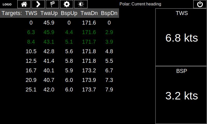
You can view the current targets table in the UI. The “active” rows of the table are highlighted in green; when the true wind speed equals one of the TWS values in the first column, that row is the exact targets. When the TWS falls between two rows (more typical), it performs a linear interpolation between them, as shown above.

When sailing to a destination that’s not directly upwind or downwind of the boat, the boat may have the choice of sailing straight at that destination rather than zigzagging (tacking or gybing, as the case may be). In this case, the VMG would be equal to the boat’s speed. But what speed should a perfectly-trimmed boat expect on an arbitrary point of sail? The Velocity Prediction Program has actually calculated the max speed achievable at all points of sail, under a range of wind conditions. The output of this is called the polars table, which is a 2-d table where rows correspond to wind speed and columns refer to degrees off the wind. Each cell gives the boat’s max speed at that wind strength and angle of attack to the wind. The targets table is just the simplified version of this that focuses on the VMG-optimal value for each row (wind speed). The app actually parses a complete polars table, which it can then visualize for you as a polar diagram:

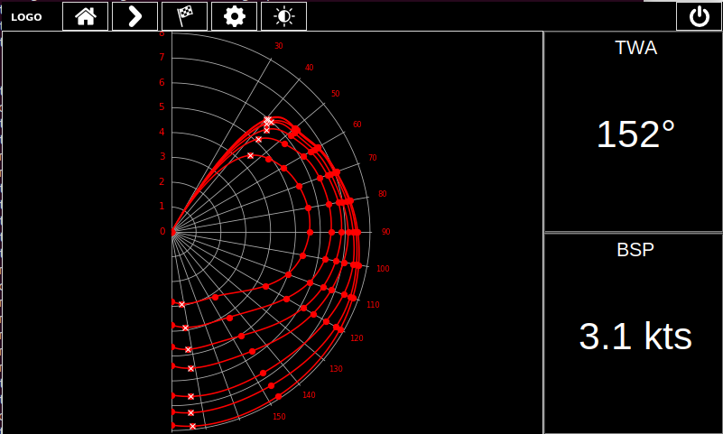
Each curve of this graph represents the boat’s maximum speed through each point of sail off the wind (straight upwind is facing up, dead downwind is facing down), at a constant wind speed. (This is true whether you’re bearing off the wind to starboard — the right — or to port — the left. The graph is shown “single sided” because the speeds on the opposite tack would just be a mirror image of this one.)

The radius at each angle is the boat speed in knots (radial axis, in knots, labeled vertically). Faster wind speeds generally correspond to higher boat speeds (greater radius), though you can see them converge to the theoretical max hull speed of the boat at which point it can go no faster. The dots are the fixed values loaded in from the table. The curves are actually spline-interpolated, which gives the expected speed for any angle and not just the pre-loaded ones. The dots with a white “X” are the max-VMG optimal angles upwind and downwind (from the companion targets table), for each wind strength line.

Doing the spline calculations was trivially straightforward thanks to SciPy and collapses to this one-liner:

spline = scipy.interpolate.splrep(angles, speeds, k=5, s=0)

The graph itself is drawn using matplotlib, which I used for a few other data visualizations as well, like tracking oscillating wind direction over time. MPL is a somewhat heavyweight graphing mechanism and I was worried about performance. But the Raspberry Pi packs pretty impressive horsepower; the longest it takes to render any data I threw at it was 120 ms. Since the polars table table never changes, that can be graphed once on startup and the image cached. But even for “real time” cases, the data does not change especially fast (N2K’s fastest update speed is 10Hz or once per 100ms), so updating a graph once every few seconds is more than enough viz responsiveness and does not overly burden interactivity.

The UI itself is built in Tk, using the tkinter python library. Tk allows for programmatic definition of GUI components; virtually every parameter of each fundamental UI widget (label, button, checkbox, etc.) can be adjusted programmatically. I really liked the Tk model; you can create literal classes to represent your particular theme styling, and then create instances of those classes for each button so they match in style. Changing the underlying class code then re-themes all the buttons together, which is much easier than changing properties in a RAD tool for several buttons one by one. The default Tk theme (at least in Raspbian’s LXDE) is… ugly. But as you can see from the screenshots, that can be entirely stripped away, to create the “flat” style shown here.

Widgets are arranged through one of a few different layout managers; they can be directly placed at specific offsets (e.g. to center an alert message); they can be arranged on a row/column grid; or given over to the “pack” layout manager that attempts to align things reasonably in a fluid way. Most of this app is built via the grid: you can pin widths and heights of some columns or rows and leave the rest floating, and it will do the right thing, or you can completely snap everything in place. I found this a very fast and logical way to build clean layouts.

By far one of the more tedious elements was the settings UI. While there are not a ton of configuration components, it still wound up being about 20% of the codebase.

App architecture

The core app is structured around two threads — one for the UI, and one for communicating with the NGT-1. Both of these are interrupt-driven; the UI thread triggers when a new UI event has occurred like a button press (which is Tk-mediated), and the I/O thread wakes when a new message is ready from the N2K bus. The UI thread also fires on a watchdog timer to periodically refresh the display (targeting 10 Hz, which is aligned with the fastest data refresh interval specified by the N2K PGNs it watches).

The UI is based around a collection of Screens; each Screen has different display and handling code. There is one screen for the main dashboard, another for the targets table display, and so on. Screens form a ring and a “next” button lets you page through them. A “home” button takes you back to the main dashboard. They’re theoretically all “drawn” on top of one another, but Tk makes it easy to hide UI elements or display others. Logical “panels” in Tk terms groups them together so you can switch the visible panel and flip between them.

The I/O thread is a loop around an InputSource and a Parser. The InputSource controls the source of new messages; this can be the NGT-1, of course, or a file to replay existing data (very useful so I don’t have to code while trying to sail at the same time). Different parsers can process the binary packet messages from the NGT-1, or one of a couple of different file formats for replay data (both binary N2K logs, and the older text-based NMEA0183 protocol). The parser has access to an object called SensorState that holds (key, value) pairs for all the variables updated by the instruments: heading, boatspeed, and so on.

Each time the parser updates some field(s), the SensorState is further updated by the math code that calculates derived values like VMG, or the updated targets for the current heading. The SensorState is also readable by the Screens, which then renders the relevant information for the user. Thanks to python’s GIL, synchronization on the thread-shared SensorState object is trivial.

To acquire files of N2K data for testing purposes, I wrote a separate program that would monitor the NGT-1 and dump all messages to a log file. Then I brought my laptop and the NGT-1 to the boat, hooked it into the network and started the logger, and sailed around for a couple of hours, putting it through a number of different paces (tacks, gybes, different points of sail, using waypoints, and so on).

There are hundreds of PGNs covering all manner of sailboat and powerboat instrument data, GPS data, engine and autopilot status, and even onboard entertainment system controls, but I ended up only needing to decode a dozen or so core PGNs for position, speed, navigation and wind information, plus time and date data for synchronizing the Raspberry Pi’s clock with the onboard network (which tracks GPS time).

Linux configuration

As mentioned earlier, Linux was configured to operate on a read-only filesystem. This required creating tmpfs mount points anywhere that needed to be written to during operation. After disabling any unnecessary services, this wound up being only /run, /tmp, a few directories under /var, and one directory specific to LXDE (the X window manager used by Raspbian).

LXDE itself was configured to launch the heads-up display app on startup, and force it to fullscreen. All system chrome (taskbars, etc.) was removed from the UI configuration. It further runs a watchdog to restart the HUD in case the app crashes.

A USB key is used for writable data storage. This includes targets or polar tables loaded in by the user, as well as the HUD configuration file that can be adjusted in the app settings. Loading in the tables is actually accomplished via WebDAV; the Pi runs nginx configured to allow you to upload files to a specific directory. The Raspberry Pi can connect to wifi and the app allows you to choose an SSID to connect to. Using your smartphone as a hotspot, you can connect the device to your phone and then drop files over through any mobile app WebDAV client.

This also provides a way to field-upgrade the device; I can upload a tarball with a particular manifest and direct the app to self-upgrade. A script will remount the root filesystem in rw mode, refresh the python code for the app from the tar file, and reboot.

I chose this WebDAV route for two reasons:

1. Because while I could have exposed an Ethernet connection through the device case, that’s one more hole where water could intrude (and more pins to corrode) — not to mention the added cost of another connector.
2. Because then I’d need to bring my laptop out to the boat to refresh the system, which is cumbersome and superfluous since it’s far more likely that I’ll have my smartphone with me anyway.

(I had originally attempted to use Bluetooth through the BlueZ BT driver for Linux, but I found it terribly unreliable and gave up.)

Math Code

The nuts and bolts of the calculations are fairly straightforward: it’s mostly trig, as taught in high school. One of the basic requirements is translating between apparent and true wind speed and direction. The apparent wind is what is experienced by the sensor itself, on a moving boat. When the boat is stationary, these are the same. But much like how a bicyclist on a windless day experiences a headwind by virtue of their own forward motion, the wind experienced by the boat is a function of the true wind and the boat’s own velocity:

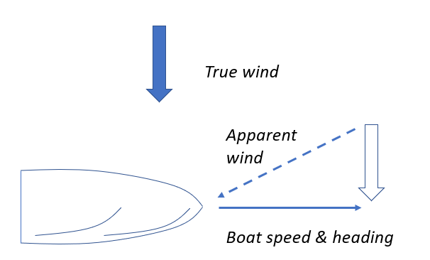
There are several great articles and blog posts such as this one by David Burch on the subject, which I used to help get things correct.

There is an arbitrary level of further depth one could get into for fine-tuning calculations about the mysteries of wind; factors like drift/leeway (the difference between your speed-through-water and speed over ground) also matter, and at the extremely fancy end, there’s the fact that the wind instrument (mounted at the top of the mast) actually experiences “twisted” wind due to an upwash effect from wind hitting the jib, rotating, and then blowing upward over the instrument. High-end racing devices use upwash correction tables to account for this. I’ve marked that as “future work” for now. But learning about these factors has helped me better understand why sometimes I don’t trust the measurements coming off the instruments exactly.

Updates on the N2K bus are being delivered by several instruments operating independently, so they may arrive in an arbitrary order. The SensorState thus retains older values until they’re overwritten, rather than operating on synchronized “frames” of input data. Some data (like wind speed) are also very “jumpy” and benefit from smoothing; otherwise it might instruct you to wildly overcorrect for a brief gust of wind. For these time series, I applied an exponentially-weighted moving average (EWMA); this function is convenient because it requires only the current measurement and previous EWMA output rather than a rolling history buffer. It also emphasizes more recent data, and older values decay gracefully out rather than in a simple moving average that treats newer and older data with equal weight.

Some simple GPIO

The main I/O with the Raspberry Pi is handled by various USB connections, and the HDMI output to the display. The Newhaven Devices display also allows you to control the brightness; especially if racing in the evening, a sunlight-readable LCD at full brightness would be too intense. A signal wire & GND connection to the LCD allow you to control the brightness by varying the duty cycle of a PWM signal.

The Raspberry Pi has a number of GPIO pins which can be configured for input or output at 3.3V. Several of its pins will also provide GND, or +5V or +3.3V power. And some pins provide for special functions, driven by the SoC itself. One of these is capable of selecting between a few hardware-driven functions, including hardware PWM output, which provides the hard real-time guarantee demanded by PWM without worrying about setting up a software thread to toggle a pin in a latency-sensitive fashion. This is accomplished on SoC pin 12, which maps to pin 18 on the Raspberry Pi 40-pin GPIO header. (It was important to note that the Broadcom BCM2837 documentation refers to pin numbering for its own IC pin-out; some of these pins are then routed to the 40-pin GPIO header on the Raspberry Pi circuit board but the numbers do not correspond directly; you need to look up the translation in the Pi documentation and double check before attaching jumper wires.)

Modifying the PWM pin state requires root privileges; I wrote a small C program that would take a value between 0 and 1024 and use that as the PWM duty cycle fraction, and invoked it via sudo to provide it the necessary privileges. The PWM capability of the BCM2837 operates by default at 1/8 of the 400 MHz base clock rate of the SoC (50 MHz). The display itself accepts PWM frequencies anywhere between 20 and 100 KHz. Fortunately, you can also set a “PWM divisor” that divides the 50 MHz clock by a constant before applying your duty cycle; applying a 1/8 divisor there runs it at about 64KHz, which is right in the middle of the acceptable range.

A brightness slider in the python app, which operates on a scale from 0 to 10 lets you adjust across the full range of backlight power from disabled to full intensity; it called the PWM helper program with sudo to adjust the power. Approximately 1/2 of the power draw (3.6W) comes from the backlight when running at full strength.

---

Most of the software development came together very quickly; I wrote the vast majority of code over a two week staycation I took around Christmas in late 2018. Choosing python made it 100x easier to get the base system together, and made it straightforward to program a pretty sharp UI. Using python libraries like SciPy and matplotlib made math handling very clean as well, and delegated the most complicated parts to a codebase that’s extremely well vetted as well as powerful. Had I tried to do this on Arduino, I wouldn’t have built nearly as many capabilities. (There are some other fun features in there like further special views for speed monitoring through tacks, and detecting wind shifts, that also leveraged these libraries.)